"What is on your mind?... What are you thinking about?... A penny for your thoughts?" For most of us, experiencing, interpreting, understanding and reacting to our own emotional states and those around us are very much a part of our daily interactions at the workplace, at home with our family members and other social settings; reacting appropriately to different situations based on the emotional context is key to developing meaningful personal and business relationships.
Appreciation of emotional context is often done in-person — and for good reason — we read emotions best based on tonality, body-language, facial expressions and many other verbal and non-verbal cues perceived both consciously and sub-consciously. For this reason, emotional interpretation is largely limited to localised settings.
But what if we could glean information on emotional responses 'en-masse' using other less conventional methods? For example, by analysing the 'tonality' of a particular writing style, or 'expressions' based on punctuation or keywords from textual input? What if we could tell how a hundred, or a thousand people are feeling at a particular point in time — in real time no less? These questions motivated my research into Natural Language Processing (NLP) and the development of a tool built on both traditional ML/NLP concepts and lexical rule-based libraries.
Problem Statement
It is difficult to gather emotional responses quickly, cheaply, and efficiently at scale.
Proposed Solution
A web-application that can process textual input to provide both a broader analysis of the emotional response to specific topics (e.g. Singapore General Elections) and a more granular analysis of sentence-level emotional responses with associated keywords and phrases.
Note: the current model is only built for text input of up to a few paragraphs long.
Use Cases for "Emotional Listening"
The following are examples of potential pain points and use cases:
Pain Points
1. Costly and time-consuming to gather mass implicit feedback: Information on emotional response to an event (a press release, a public speech) could inform better decision-making, but obtaining implicit feedback in real-time at scale is often prohibitively expensive. While explicit feedback can be obtained from social media platforms (e.g. Facebook emoji reactions), this only captures a secondary reaction. It would be more powerful to get an implicit primary reaction from people's own textual input on public platforms.
2. Difficult to obtain real-time information to take preventive action: Unfortunate events like mass-killings are often preceded by telling messages indicative of troubled emotions — but are usually only discovered post-mortem.
3. Lack of nuance in basic sentiment analysis: Current sentiment analysis is usually binary (positive/negative). However, even within the category of "negative," the appropriate response varies widely: disappointment that a product feature wasn't released is very different from anger that a product is dangerous. Granular emotion classification enables more appropriate responses.
Use Cases
- Emotional analysis as an additional data point for digital marketing
- Better recommendation systems (think: Spotify playlist suggestions that match your current mood)
- Real-time "emotional listening" to pre-empt bad events — dynamically scraping a live source and generating real-time emotion breakdowns
- More granular sentiment analysis for policy makers
- Mental health tracker: individuals can journal and track their emotional state over time
- Assistive technology for disabilities: combined with speech-to-text, this could help those with impaired ability to pick up emotional nuances in daily interactions
1. Data Cleaning and Pre-Processing
1.1 Combining 3 Datasets
Three pre-tagged datasets were combined:
- Kaggle dataset (~415,000 tweets): tagged across 6 emotions — sadness, joy, love, anger, fear, surprise
- Figure Eight dataset (~40,000): 13 emotions including neutral, enthusiasm, hate, boredom, relief
- Figure Eight dataset (~2,500): 18 emotions including anticipation, aggression, contempt, disapproval, remorse
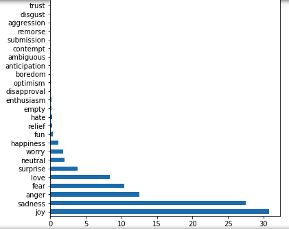
1.2 Problem of Imbalanced Data
There was clearly a long tail of more nuanced emotion types with far fewer observations than "plain vanilla" types like joy and anger. This imbalanced dataset would impact prediction accuracy. I chose to subset only the top 8 emotions by count to form the final training dataset.
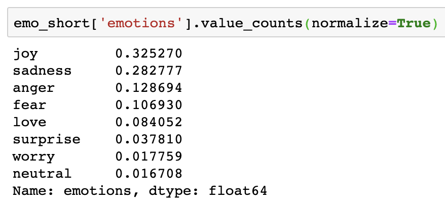
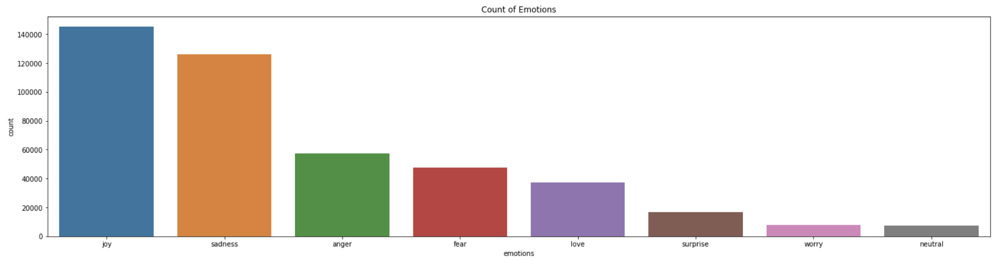
Even after shortlisting the top 8 emotions, significant class imbalance remained. I addressed this using random upsampling within each emotion class after train-test-split, to prevent the same observations from appearing in both training and testing sets.
1.3 Text Cleaning Function
A custom cleaning function strips non-letters, converts to lowercase, removes stopwords, and lemmatises:
from bs4 import BeautifulSoup
import regex as re
from nltk.corpus import stopwords
from nltk.stem import WordNetLemmatizer

lemmatizer = WordNetLemmatizer()

def clean_text(raw_post):
    # 1. Remove HTML
    review_text = BeautifulSoup(raw_post).get_text()

    # 2. Remove non-letters
    letters_only = re.sub("[^a-zA-Z]", " ", review_text)

    # 3. Convert to lower case, split into individual words
    words = letters_only.lower().split()

    # 4. Convert stop words to a set (faster lookup)
    stops = set(stopwords.words('english'))

    # 5. Remove stop words
    meaningful_words = [w for w in words if not w in stops]

    # 6. Lemmatise
    lem_meaningful_words = [lemmatizer.lemmatize(i) for i in meaningful_words]

    # 7. Join words back into one string and return
    return(" ".join(lem_meaningful_words))
There were 5,519 values (1.22% of observations) that turned up null after cleaning — we still had 98% of our dataset to work with.
1.4 Cleaning Difficulties
- Selectively keeping special characters that convey useful information (e.g. emojis)
- Removing or contracting words with character repetitions (e.g. "whaaaaaat" → "what")
- Transforming contractions to normal forms (e.g. "can't" → "cannot")
- Removing stop words while maintaining negations (e.g. "not", "no") to preserve intention
- Separating concatenated words (e.g. "iloveyoutodeath")
- Correcting misspellings
- Stripping usernames (e.g. @XYZ)
2. Baseline Model
2.1 Train-Test-Split
from sklearn.model_selection import train_test_split
X = emo_short['clean_text']
y = emo_short['emotions_label']
X_train, X_test, y_train, y_test = train_test_split(
X, y,
test_size=0.25,
random_state=42
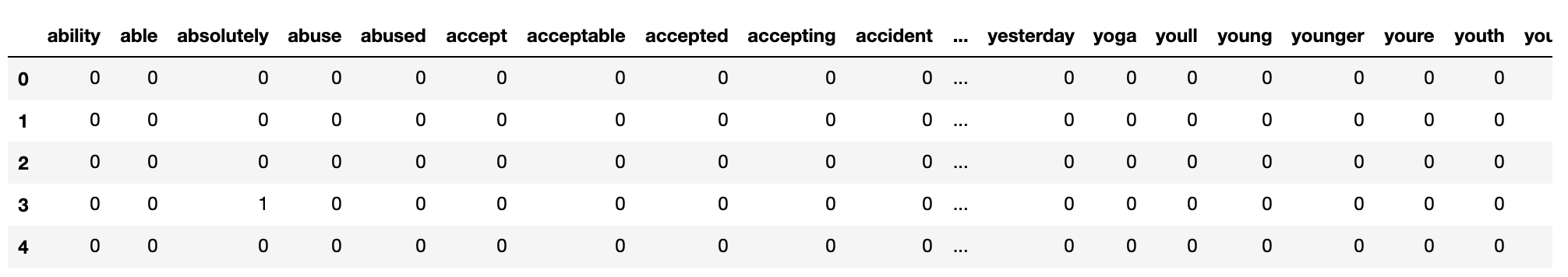
)2.2 Vectorising Word Features
There are two main vectorisers: CountVectorizer (counts occurrences of each unique word) and TF-IDF Vectorizer (assigns a score based on how distinctive a word is across the corpus).
Without restricting the number of word features, the total unique vocabulary exceeded 70,000 words. With ~350,000 training rows, the full sparse matrix would contain over 23 billion cells — my kernel crashed attempting this. I limited to 2,000 features with a minimum document frequency of 10.
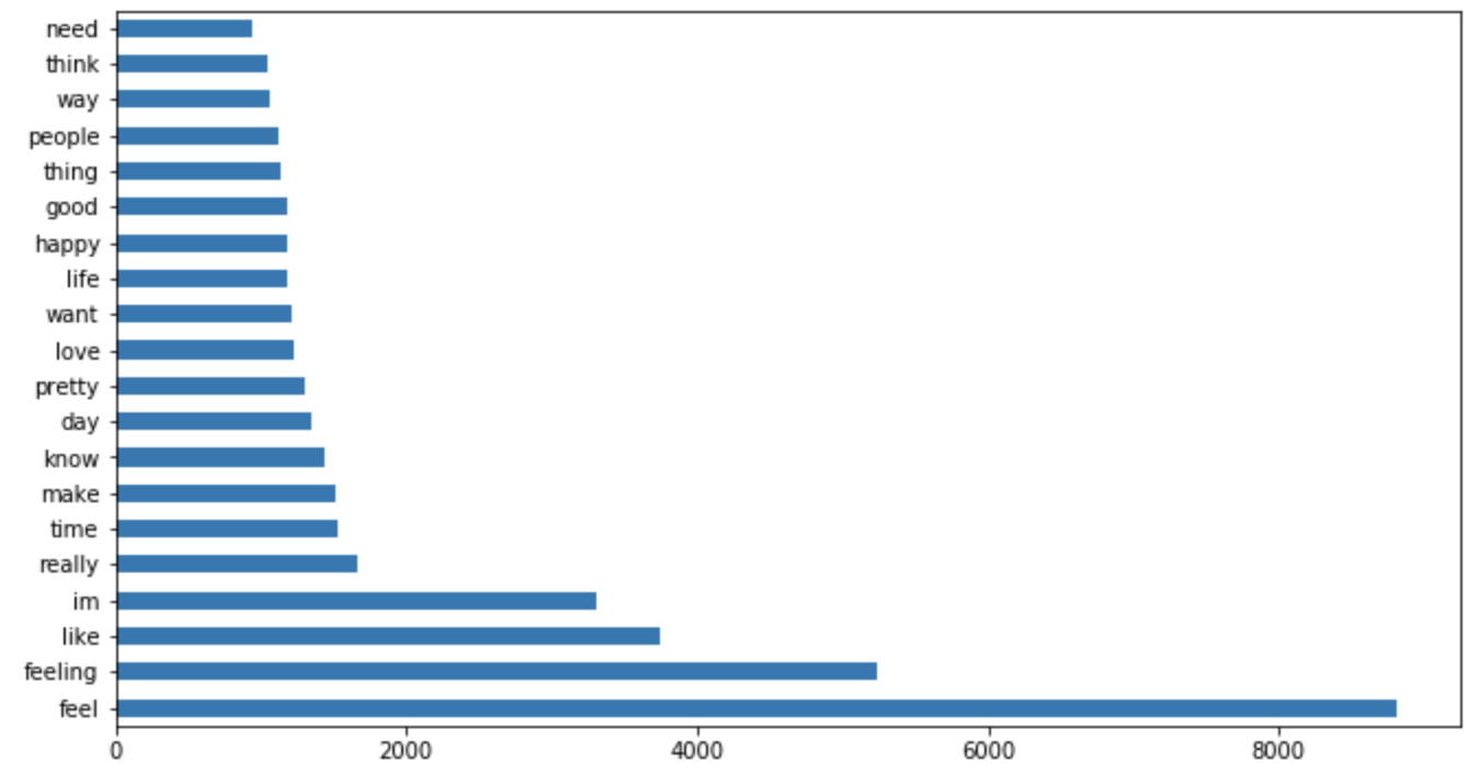
Finding the most frequently used words per emotion:
joy_df = train_cvec_combined_df[train_cvec_combined_df['emotions_label']==2]
joy_df.drop('emotions_label', axis=1, inplace=True)
top_20_joy = joy_df.sum().sort_values(ascending=False).head(20)
top_20_joy.plot.barh(figsize=(11,6));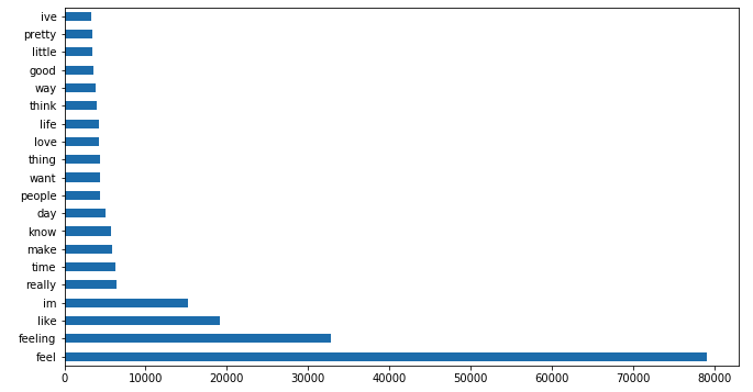
A key observation: there were many overlapping high-frequency words across the 8 emotion classes (e.g. "im", "feeling", "feel", "know", "day") — not particularly informative for distinguishing emotions. Only 36.8% of top-20 words across all classes were unique.
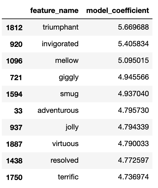
By contrast, the words with the highest model coefficients were much more distinctive:
2.3 Baseline Model Results
Used CountVectorizer + Logistic Regression:
lr = LogisticRegression(max_iter=400000)
baseline_model = lr.fit(X_train_cvec, y_train)| Metric | Score |
|---|---|
| K-fold CV (mean) | 0.848 |
| Train accuracy | 0.865 |
| Test accuracy | 0.849 |
The K-fold scores are consistent across 5 folds, and the train/test gap is small — the model is not overfitted. Overall, strong results.
3. Tuning and Alternative Models
TF-IDF Vectorizer
Surprisingly, TF-IDF's top words were similar to CountVectorizer's, and the model performed slightly worse:
| Metric | Score |
|---|---|
| Train accuracy | 0.848 |
| Test accuracy | 0.841 |
Naive Bayes (Grid Search)
Used a pipeline with GridSearchCV across 4 model/vectorizer combinations and 96 parameter combinations:
from sklearn.naive_bayes import BernoulliNB, MultinomialNB
from sklearn.pipeline import Pipeline

models1 = {
    'TVEC + Bernoulli': Pipeline([("vec",TfidfVectorizer()),("nb",BernoulliNB())]),
    'TVEC + Multinomial': Pipeline([("vec",TfidfVectorizer()),("mb",MultinomialNB())]),
    'CVEC + Bernoulli': Pipeline([("vec",CountVectorizer()),("nb",BernoulliNB())]),
    'CVEC + Multinomial': Pipeline([("vec",CountVectorizer()),("mb",MultinomialNB())])
}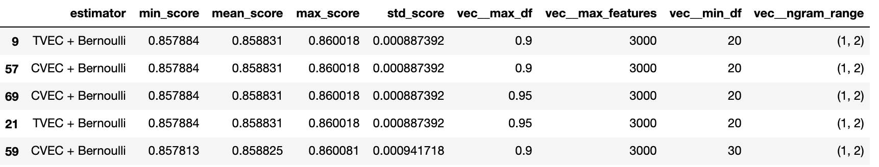
The top score goes to TVEC + Bernoulli at 0.858, but the improvement over the baseline is marginal. The optimal parameters were consistently n-gram range (1,2) and max_features = 3,000 — intuitive, as larger n-gram ranges better capture context and more features provide more signal.
Random Forest and Extra Trees
| Model | Train score | Test score |
|---|---|---|
| Random Forest (10 trees) | 0.947 | 0.808 |
| Extra Trees (10 trees) | 0.951 | 0.811 |
Both are heavily overfitted (large train/test gap) and perform worse than the baseline. With more trees they might improve — but the computational cost is prohibitive for ~500k rows.
Artificial Neural Network
from keras.models import Sequential
from keras.layers import Dense

nn_model = Sequential()
nn_model.add(Dense(256, input_dim=n_input, activation='relu'))
nn_model.add(Dense(n_output, activation='softmax'))
nn_model.compile(loss='categorical_crossentropy', optimizer='adam', metrics=['accuracy'])
Two ANN configurations were tried. Both achieved ~0.85 validation accuracy — equivalent to the baseline — and the simpler model began overfitting after 1.5 epochs. No improvement over Logistic Regression.
4. Model Selection
After testing six approaches — Logistic Regression (CVEC/TVEC), Naive Bayes (Multinomial/Bernoulli), Random Forest, Extra Trees, SVM (abandoned — too slow), and ANN — the baseline CountVectorizer + Logistic Regression was selected.
5. Lexical Rule-Based Libraries for Sentiment Analysis
In addition to emotion classification at the sentence level, I wanted to contextualise those emotions using lexical libraries to provide valence scores and highlight key phrases associated with the classified emotion.
VADER (Valence Aware Dictionary and sEntiment Reasoner)
VADER is "a rule-based sentiment analysis engine incorporating grammatical and syntactical rules, including empirically derived quantifications for the impact of each rule on perceived sentiment intensity." It goes beyond bag-of-words by handling emoticons, capitalisation, punctuation, and word order.
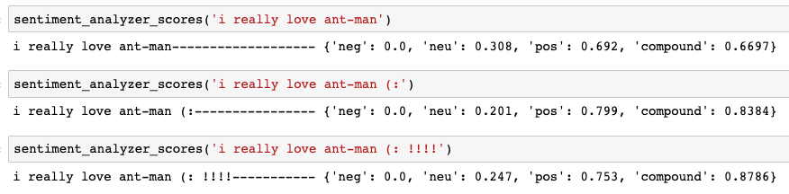
How VADER adds context:
- Valence vs. emotion: Valence measures the intrinsic positivity/negativity of a word or phrase, independent of the specific emotion. For example, "I think you are a racist person" carries a negative valence without clearly indicating the speaker's emotion.
- Emotional intensity: Two sentences classified as "angry" may differ significantly in intensity — the more negative valence score indicates more intense anger.
- Model validation: Valence scores should correlate with classified emotions (negative valence for sadness/anger/fear). Mismatches flag potential misclassifications.
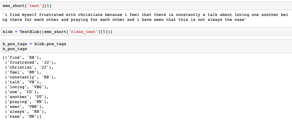
TextBlob
TextBlob was used for noun-phrase extraction and part-of-speech (POS) tagging to identify adjectives and verbs associated with the classified emotion.
6. Combining Functions for Deployment
The emo_machine() function combines the full pipeline: takes in raw text, tokenises into sentences, cleans for the ML model while keeping raw text for VADER (which works better on uncleaned text), runs classification, VADER scoring, and TextBlob extraction, and returns a sorted dataframe.
def emo_machine(text_string_input):

    emo_summary = pd.DataFrame()
    vader_scores = []
    bnp = []
    b_pos_tags = []
    pos_subset = ['JJ']  # adjectives only

    # Load pickled model artifacts
    pickle_in = open("lr_baseline_model","rb")
    lr_baseline_model = pickle.load(pickle_in)
    pickle_in = open("cvec","rb")
    cvec = pickle.load(pickle_in)
    pickle_in = open("clean_text","rb")
    clean_text = pickle.load(pickle_in)

    # Tokenise input into sentences
    text_input_sent = nltk.tokenize.sent_tokenize(text_string_input)

    # Clean each sentence for ML model
    clean_text_input_sent = [clean_text(i) for i in text_input_sent]

    # Vectorise and predict emotions
    X_input_cvec = cvec.transform(clean_text_input_sent).todense()
    predictions = lr_baseline_model.predict(X_input_cvec)

    # VADER scores on RAW text (not cleaned)
    for sent in text_input_sent:
        vader_scores.append(vader.polarity_scores(sent)['compound'])

    # TextBlob noun-phrases and POS tags on cleaned text
    for sent in clean_text_input_sent:
        blob = TextBlob(sent)
        bnp.append(blob.noun_phrases)
        sent_pos_tags = [word for word, tag in blob.pos_tags if tag in pos_subset]
        b_pos_tags.append(sent_pos_tags)

    emo_summary['emotions'] = predictions
    emo_summary['sentences'] = text_input_sent
    emo_summary['vader_scores'] = vader_scores
    emo_summary['blob_phrases'] = bnp
    emo_summary['blob_tags'] = b_pos_tags

    return emo_summary.sort_values(by=['vader_scores'], ascending=False)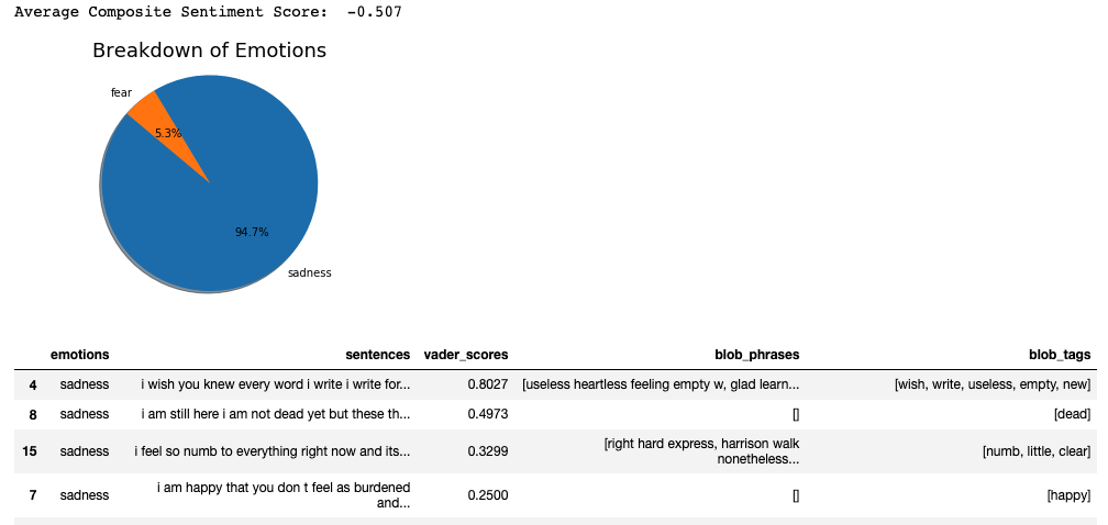
7. Flask Deployment
The function was wrapped in a Flask application with two routes: a home page for text input and a results page that generates the emotion breakdown.
app = Flask(__name__)

@app.route('/')
def index():
    form = ReviewForm(request.form)
    return render_template('reviewform.html', form=form)

@app.route('/results', methods=['POST'])
def results():
    form = ReviewForm(request.form)
    if request.method == 'POST' and form.validate():
        review = request.form['moviereview']
        emotions = emo_machine(review)[0]
        return render_template('results.html',
                            content=review,
                            tables=[emotions.to_html()],
                            titles=['emotional breakdown'],
                            score=emo_machine(review)[1])
    return render_template('reviewform.html', form=form)
8. Heroku Deployment
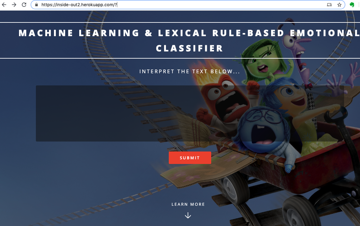
Note: The Heroku free tier has since been discontinued — the live link is no longer active. The code is available on GitHub.
Post-Mortem: Improvements and Reflections
Model Improvements
- More rigorous class balancing in the dataset
- Long Short-Term Memory (LSTM) / Recurrent Neural Networks for better sequential context
- Gensim and spaCy for aspect mining and named entity recognition
- Manually curate and extend VADER's lexical library with local (Singaporean) lexicon
UI/UX Improvements
- Interactive visualisations — clickable graph elements, sentence highlighting linked to emotions
Deployment Improvements
- Link to a database with a feedback button to continue collecting classification accuracy data
- Dynamic scraping from a chosen source (e.g. a Twitter feed) to track emotions over time
Other Reflections
- Text as a single reference point for emotion loses verbal intonation, facial expressions, etc.
- A single sentence can contain multiple emotional states — how many should be classified?
- Sarcasm and passive-aggressiveness are extremely difficult to detect reliably.
- Pejoratives (neutral-sounding statements that mask negativity: "his idea was interesting") are hard to catch.
- Slang is localised and dynamic — models trained on American social media won't generalise to Singaporean colloquialisms. The lexicon needs continuous updates.
- Lexical methods are context-specific — social media vs. formal prose would require different training data.